- Published on
Deriving Neural Networks

Neural networks encompass a wide array of predictive algorithms that are the backbone of many of the latest advances in artificial intelligence and machine learning. I'm going to explain and derive the math behind a very basic type of neural network — a single hidden layer neural network.
Notation & Symbols
The goal of a neural network is the same as any other supervised learning technique. We have a series of predictors or input data, , and are trying to predict a response(s), . is a matrix consisting of columns where each column represents a different predictor variable. is a vector consisting of classes.
| ... | |||
|---|---|---|---|
| ... | |||
| ... | |||
| ... | ... | ... | ... |
| ... |
The subscript represents the row from where is the number of rows i.e. data points in our dataset. The subscript represents the column from where is the number of columns i.e. the variables in our dataset. If we had 3 variables consisting of age, gender, and height as well as 3 observations for each variable then the above table would look like the following:
| age | gender | weight |
|---|---|---|
| 18 | M | 177 |
| 24 | M | 164 |
| 44 | F | 159 |
For the above table, and . Now, is a matrix of responses.
| ... | |||
|---|---|---|---|
| ... | |||
| ... | |||
| ... | ... | ... | ... |
| ... |
Again, the subscript represents the row from and is the column i.e. class from . Let's say we are trying to predict salary from age, gender, and weight. Since we are only trying to predict 1 response, that means we have classes. So, the above table is simplified to:
| salary |
|---|
| 60,000 |
| 39,000 |
| ... |
| 121,000 |
Hopefully, you now understand the notation behind representing the data. It's important to remember the above notation or things will get very confusing.
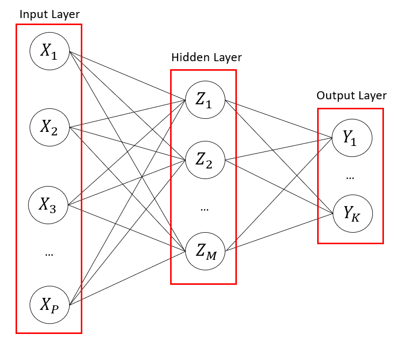
Network Diagram
We represent neural networks using a network diagram.
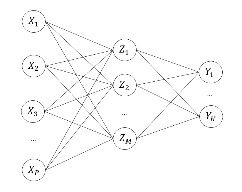
Network diagrams help us visualize the input layer, hidden layer(s), and the output layer. The input layer consists of nodes that represent our input variables, . The hidden layer consists of hidden nodes which we'll represent as where . The output layer represents the classes or responses, . The lines inbetween nodes represent our connections between the nodes. In a basic neural network, each node in a layer is connected to all of the nodes from the previous layer. For example, the hidden node receives connections from .
The middle layer is called the hidden layer because we don't directly observe their values. In a neural network, all we really "see" are the values for the inputs and the values for the outputs. In a single-layer hidden neural network, we only have 1 hidden layer. Multi-layer neural networks have multiple hidden layers.
Forward Propagation
I'll be using the same notation that is used in Elements of Statistical Learning textbook. Each node in the hidden layer represents a linear combination of the inputs. Let's start with the inputs:
The lines in the above network diagram represent different linear combinations.
The and are called the bias and weights, respectively. Each hidden node, , has a different value for bias and weight. The bias term, , is a single value while the weights is a vector of length (the number of input variables). The superscript means we take the transpose of the weight vector. Each weight in our weight vector represents how much we need to scale our respective input variable, .
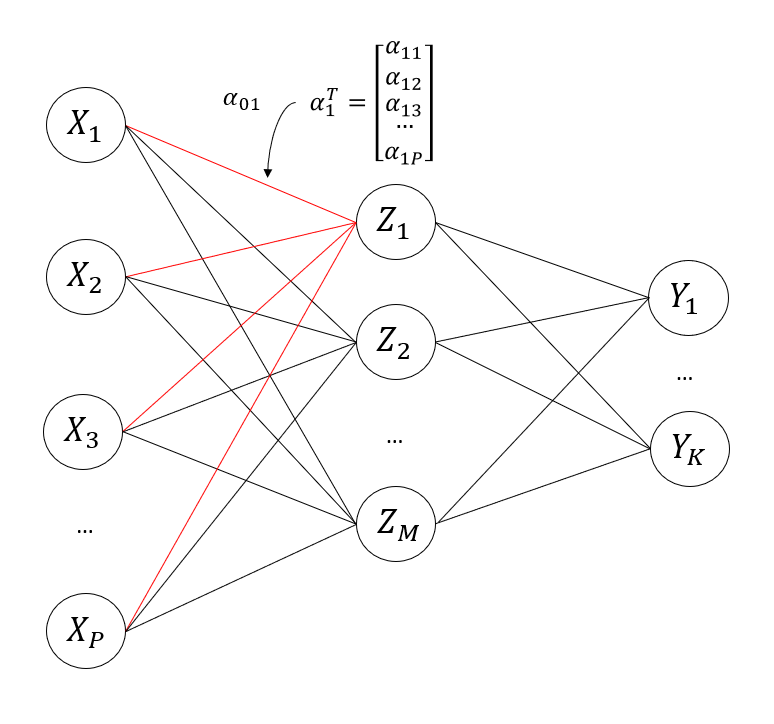
After we create a linear combination, the hidden node then applies an activation function, :
Now we need to transform our values into the output. To do this, we take another linear combination except this time its of the values.
Remember that represents which output node we are dealing with. If we only have 1 output node, then . The symbol again represent our weights and biases. We use a different symbol for them here to show that these are the weights and biases specifically for transforming the values in our hidden nodes to the output nodes.
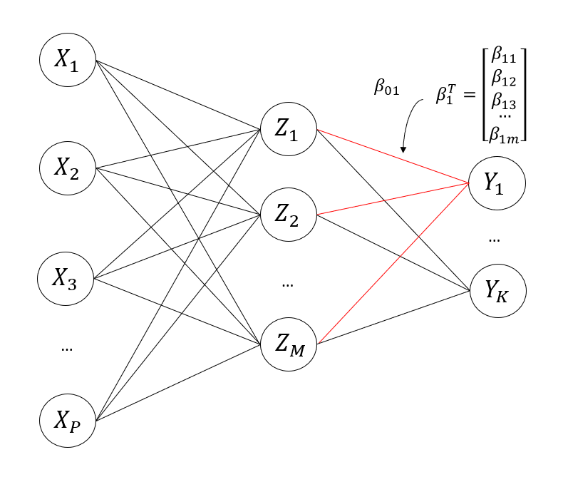
Now, our output is equal to:
Now, our output depends on whether we are dealing with a regression or classification problem. If we are dealing with regression, then our output is simply equal to .
When making predictions for a classification problem, we need to use the softmax function to transform the values into values between 0 and 1.
The above gives us an array of size . The class with the largest value (between 0 and 1) is our class prediction.
Back Propagation
Fitting a neural network to a certain dataset involves finding the optimal values for the weights and biases. The optimal value is that which minimizes the loss function. For regression problems, the loss function is the Residual Sum-of-Squares (RSS):
For the sake of simplicity, we'll combine the respective bias and weights into a single term. So we have:
We need to use gradient descent to update and find the optimal values for the above weights.
The constant, , is the learning rate and is usually a small value like 0.01. Let's calculate the derivatives for each respective weight:
As seen in the forward propagation section, , so we can rewrite the above equation as:
We can split the partial derivative further since :
We will simply rewrite as . We can also see that .
We write as to indicate the -th node and the -th observation. In the case where , the remaining derivative is just 1. Now, we follow a similar procedure for the other weights, :
That's all we need to compute the gradient descent to update our weights! For classification, we use the cross-entropy loss function and the derivations can be found in the same way.