Machine Learning Part 2: Loss Functions & Convexity
Authors
Name
Jyotir Sai
Twitter
Engineering Student
Loss functions tell us how far our predicted value is from the ground truth.
What are some important properties that loss functions should have? Why do we
use squared error loss functions? The purpose of this blog is to answer those questions.
Before diving into loss functions and convexity, I want to talk about the math notation
we'll be using.
Vector Representation
The input matrix, X, can be written as:
X=⎝⎜⎜⎜⎛−x(1)−−x(2)−...−x(M)−⎠⎟⎟⎟⎞ϵRM
In the above representation, each row vector corresponds to a sample and we have M samples/rows.
The values in this vector are an element of the RM space because if we have M samples
then we have M dimensions. The values in a single row vector correspond to each feature i:
x(1)=[x1(1),x2(1),...,xi(1)]
x(2)=[x1(2),x2(2),...,xi(2)]
...
x(M)=[x1(M),x2(M),...,xi(M)]
It is also common to write the matrix with the rows as features and columns as samples:
X=⎝⎛∣x(1)∣∣x(2)∣...∣x(M)∣⎠⎞
In machine learning, we usually use matrices / vectors to represent our variables so we
can take advantage of vectorization.
Let's talk about how to use linear regression when dealing with vectors.
The equation for linear regression with a matrix of input values is written below.
h(X)=wTX+b
Instead of a single slope value, we have a vector of values, w, known as the weights.
w=⎝⎜⎜⎜⎛w1w2...wi⎠⎟⎟⎟⎞ϵRi
Each corresponding input feature xim, has a corresponding weight wi. The y-intercept, b, is still represented with b except we call
this term the bias.
For aesthetic reasons, the bias term is sometimes absorbed into the weight vector so we can write:
The above vector representation is the same as writing:
h(x)=b+w1x1+w2x2+...+xdwd
Loss Function
We previously discussed the squared error loss function:
J=21m=1∑M(ym−h(xm))2
Another loss function we can use is the mean squared error:
J=M1m=1∑M(ym−h(xm))2
Now, let's express the loss function in a matrix-vector form. The L2 norm of a vector is
defined as:
∥ν∥2=i=1∑dνi2
The L2 norm can be used to express the summation term in the loss function in vector form:
m=1∑M(ym−h(xm))2→∥y−h∥2
As seen above, h is simply equal to wTX.
∥y−h∥2→∥∥∥y−wTX∥∥∥2
The matrix-vector version of the mean squared error is therefore:
J=M1∥∥∥y−wTX∥∥∥2
or
J=M1∥Xw−y∥2
Why do we use these loss functions in particular? Why do we square the error instead of cubing it
or raising it to a higher power? Since we want the minimum of a loss function, we want to differentiate
the loss function and find where its derivative is 0. Therefore, we want to choose a loss function that is differentiable. We also want a loss function where the point at which the derivative is 0
corresponds to the global minimum. More formally, we want a loss function that is both smooth and
convex.
Convex Sets
Before talking about convex functions, we'll first have to cover convex sets. A set, S, is convex if and only if
∀x,yϵS,∀λϵ(0,1)
λx+(1−λ)yϵS
In plain english, the above means that for all x,y that are an element of S, and for all λ values between 0 and 1, the equation on the second line yields a value that is also apart of the set.
Let's look at some visual examples.
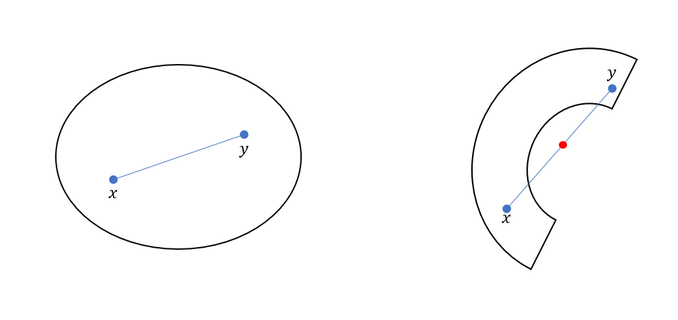
The example on the left is a convex set because for all points x and y, the line that connects them will always be inside the set. The example on the right is not a convex set since the
line between x and y goes outside of the set. Our value of λ picks a point on this line. For example, λ=0.5 results in the red point in the middle of the line.
λx+(1−λ)y=0.5x+(1−0.5)y=21(x+y)
Simple sets like the empty set, lines, and hyperplanes are all considered convex. Discontinuous sets are not convex.
Convex Functions
A real-valued function, f, is convex if the domain of f is a convex set. For all x and y in the domain of f, and for all λϵ(0,1), we have
the following relation
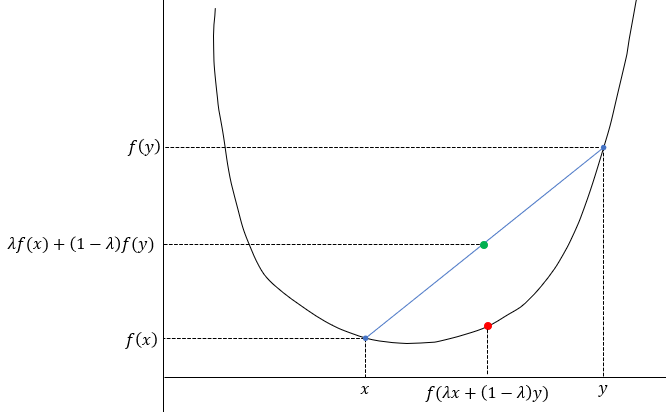
λf(x)+(1−λ)f(y)≥f(λx+(1−λ)y)
The above relation holds true for a convex function.
A quadratic is a convex function, so the green point will always lie above the red point. The line
between the points f(x) and f(y) will always lie above the function f.
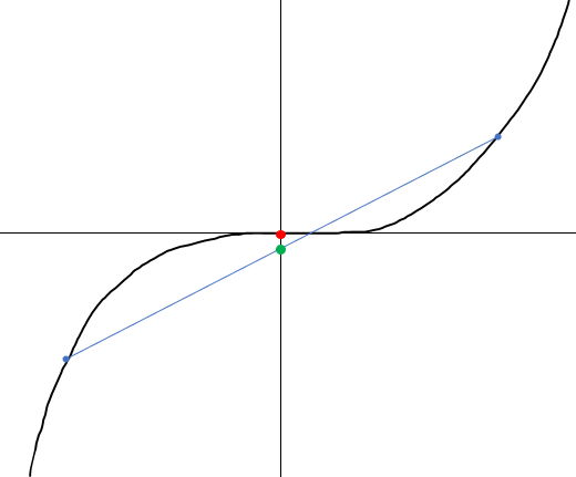
The cubic function shown above is not a convex function since the green point lies below the red point,
violating the above relation.
There are two more properties of convex functions that you should know. Let's
start with the 1st-order condition which states that for all x,y in the domain of f
f(y)≥f(x)+∇xf(x)T(y−x)
The term on the right is the 1st-order Taylor polynomial expansion where
∇xf(x)=⎝⎛∂x1∂f(x)...∂xi∂f(x)⎠⎞
Let's again look at a visual example.
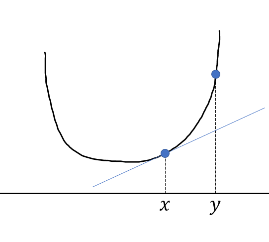
The blue line is the 1st-order Taylor expansion (tangent line). According to the 1st-order condition, this line
will never cross "inside" the function. It will always be less than or equal to f(y). All the points
on the graph are "above" the tangent line.
The 2nd-order condition states that
∇x2f(x)≥0
where ∇x2f(x) is the Hessian matrix.
The 2nd-order condition says that if the 2nd-order derivative of a function is greater than or equal to 0 (positive semi-definite),
then the function is convex. A matrix is positive semi-definite if its eigenvalues are greater than or equal to 0.
To summarize, if a function, f, is twice differentiable, then the following conditions are equivalent.
λf(x)+(1−λ)f(y)≥f(λx+(1−λ)y) (f is convex)
f(y)≥f(x)+∇xf(x)T(y−x)
∇x2f(x)≥0
Revisiting Loss Functions
We previously looked at the mean squared error loss function:
J=M1∥Xw−y∥2
We add a factor of 1/2 to the above function so that when we take the derivative it cancels
out the 2 from the exponent. It is done purely for aesthetic reasons.
J=2M1∥Xw−y∥2
Now, let's work on finding the derivative for this function. The L2-norm can be rewritten as
J=2M1(Xw−y)T(Xw−y)
Remember that (AB)T=BTAT
J=2M1(wTXT−yT)(Xw−y)
J=2M1[wTXTXw−wTXTy−yTXw+yTy]
Inside the brackets, the two terms in the middle are actually the same since
yTXw=(yTXw)T=wTXTy
The above term actually results in a scalar, that's why it's equal to its transpose.
J=2M1[wTXTXw−2yTXw+yTy]
Taking the derivative
∂w∂J(w)=2M1[2XTXw−2XTy]
The above derivative uses the following identities
∂x∂xTSx=2Sx
∂x∂Ax=AT
Where S=XTX and A=yTX. The yTy term has no w term so its derivative is just 0. The derivative
can be further simplified to
∂w∂J(w)=M1XT(Xw−y)
Taking the 2nd derivative
∂w2∂2J(w)=∇w2J(w)=M1XTX
We want to know whether the above equation satisfies the 2nd-order condition (∇w2f(w)≥0).
How do we tell whether the matrix XTX is positive semi-definite? A matrix M is positive
semi-definite if the number produced by zTMz is non-negative where z is a nonzero column vector.
zT(XTX)z
(Xz)T(Xz)=∥Xz∥2≥0
The above shows that the mean-squared error function is indeed convex.