Machine Learning Part 5: Bias-Variance Trade-off

In the previous blog post, we saw that estimating parameters using maximum likelihood estimation is equivalent to using the mean squared error.

The above estimate for $\mathbf{w}$ is said to be an unbiased estimate for the weight. A parameter is said to be unbiased if the expectation is equal to the true value of the parameter. We can easily prove that this is the case

I've simply plugged in the closed-form solution for $\mathbf{w}$ that was derived in part 3. When we started the maximum likelihood estimation, we assumed our model was

We can vectorize the above equation and plug it in for $\mathbf{Y}$

We assumed that the error, $\epsilon$, has a mean of zero therefore the expectation of the second term is just 0. The 1st term can be reduced to

We've now seen that the expectation of $\mathbf{\hat{w}}$ is equal to the true value $\mathbf{w}$. Therefore, the parameter estimated by maximum likelihood estimation is said to be unbiased and has the least variance.

Bias-Variance Decomposition

Let's assume we have the following model

where $f(x)$ is some unknown function with zero mean noise. Given a hypothesis, $h$, we can quantify how good our estimate is by using the squared error

The average error is the expectation over the squared error which is also known as the risk

Plugging in our equation for $y$

Expanding terms

Since $\epsilon$ has an expectation of zero, the last term is simply zero.

Now we will take the expectation over all training datasets $D$

We will use the term $\mathbb{E} \left [h'(x) \right]$ to denote the average prediction over every training set. We're going to add and subtract this term below

Expectation is linear so we can expand into

Let's look at the 3rd term more closely

Neither of the terms in $\left[\mathbb{E} \left [h'(x) \right] - f(x) \right]$ actually depend on the dataset so it can simply be written as

Now we'll distribute $\mathbb{E}_{D}$

As we saw above, the term $\mathbb{E}\left [h'(x) \right]$ does not depend on the dataset. The term $\mathbb{E}_{D} \left[h(x) \right]$ is just equal to $\mathbb{E}\left [h'(x) \right]$, so the terms just subtract each other out

The final equation for the expectation of the risk is now

The first term in the above equation is what we call the variance. The second term is the bias and the last term is the noise.

The noise is also known as the irreducible error. Therefore, in machine learning when we minimize the mean squared error, we are really trying to minimize the variance and bias. What do we actually mean when we say variance and bias? Variance describes the error from applying our model on the test set. If our training set error is low but our test set error is high then we have high variance. Bias refers to the error between the true underlying function that describes the data and our model. If our training set error is high then have a bias problem. Let's explore these concepts further.

Bias-Variance Intuition

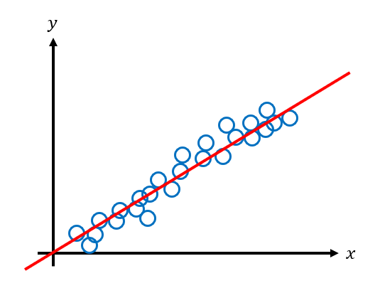
Bias and variance play an important role in developing machine learning models. They are easier to explain with visual examples. Let's say we have the following data that we want to fit a machine learning model to.

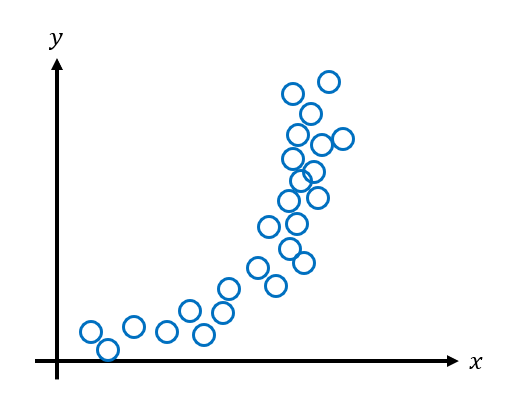
The data looks quadratic so let's use a quadratic model to fit the data.

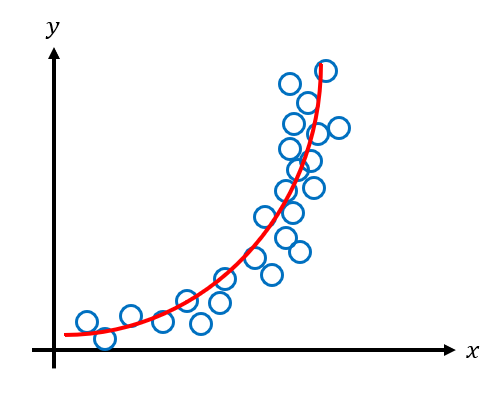
The model fits the data pretty well. We can see that the error between our model and the data is quite low i.e. it has low bias. How does the model perform with data it has never seen before? Let's say our test data looks like the following.

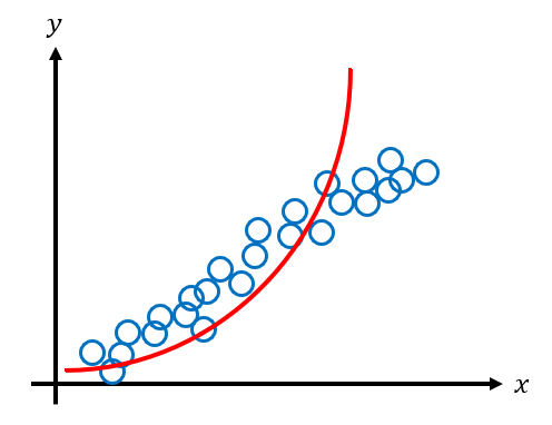
The model doesn't fit the test data as well as the training data, particularly towards the later data points. When this happens, we say that the model does not generalize well. Models that don't generalize well have high variance. To lower the variance and improve generalization, it's often better to use a simpler model. For example, instead of using a quadratic model we can use the simpler linear model.

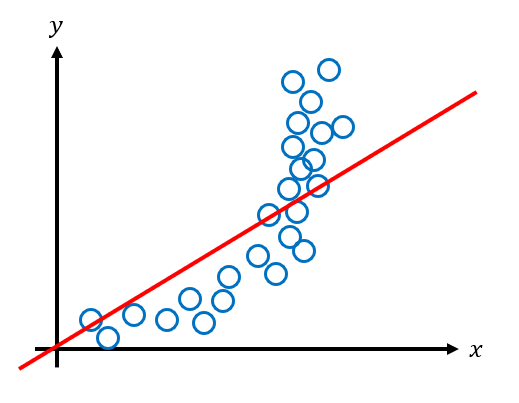
The linear model clearly doesn't fit the original data as well as the quadratic model, but how does it perform on the test set?

The linear model performs much better on the test data. It generalizes better in this example since it does not overfit to the original data. This model has high bias but low variance.

When we overfit to the training data we have low bias but high variance. When we underfit to the training data we have high bias but low variance. This is the essence of the bias-variance tradeoff. We need to find the optimal model that minimizes both the bias and the variance, and therefore the total error.

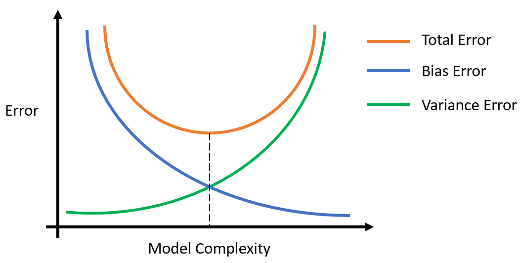
The above graphic summarizes the bias-variance tradeoff. As our model gets more complex (i.e. more parameters), the bias error becomes smaller while the variance error becomes larger. The total error decreases until a minimum is reached, and then it starts increasing again as the model becomes too complex and suffers from variance. Regularization involves taking a complex model and simplifying it to reduce variance. There are a couple different methods to achieve this which we'll talk about in the next blog post.