Machine Learning Part 3: Optimality & Gradient Descent

In part 2 of this series, I briefly mentioned local versus global minimums and how we want the global minimum of a function. What are local and global minimums? How do we get the global minimum? In this blog post, I'll be covering local and global minimums as well as a numerical technique called gradient descent which allows us to reach the minimum.

Local versus Global minimum

Let's say we're looking at a range, $(a, b)$ , in a function, $f$ , and $(x, f(x))$ is a point in that range where $a < x < b$ . The point, $(x, f(x))$ , is a local minimum if $f(x) \leq f(y)$ for every $y$ in the range $(a,b)$ . It's easier to understand this jargon with a visual example.

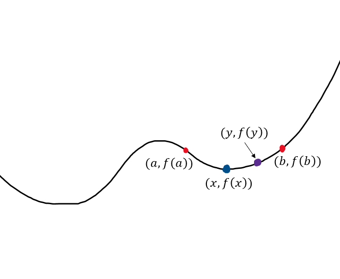
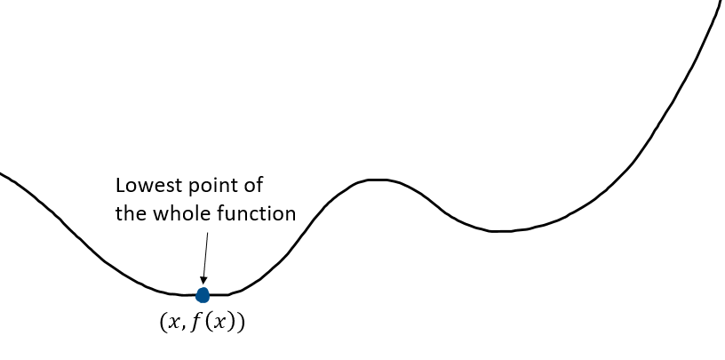
The point $(x,f(x))$ is the lowest point in the range $(a,b)$ therefore it is called a local minimum. The global minimum is the point, $(x, f(x))$ , where $f(x) \leq f(y)$ for all $y$ in the entire range of $f$ .

For a convex function, the local minimum is the global minimum. A minimum (or maximum) occurs wherever the derivative is equal to 0.

Minimizing MSE function

In part 2 of this series, we saw the mean squared error loss function along with its 1st and 2nd derivatives.

J \left(\mathbf{w} \right) = \frac{1}{2M} \left \| \mathbf{X}\mathbf{w}-\mathbf{y} \right \|^{2}

\nabla J(\mathbf{w}) = \frac{1}{M} \mathbf{X}^{T} \left (\mathbf{X}\mathbf{w}-\mathbf{y} \right)

\nabla^{2} J(\mathbf{w}) = \frac{1}{M} \mathbf{X}^{T} \mathbf{X}

When training a machine learning model, we want the value of $\mathbf{w}$ that minimizes $J(\mathbf{w})$ . We already saw that MSE is a convex function so wherever the 1st derivative is equal to zero gives us the optimal value for $\mathbf{w}$ .

\nabla J(\mathbf{w}) = \frac{1}{M} \mathbf{X}^{T} \left (\mathbf{X}\mathbf{w}-\mathbf{y} \right) = 0

\mathbf{X}^T\mathbf{X}\mathbf{w}-\mathbf{X}^T\mathbf{y} = 0

\mathbf{X}^T\mathbf{X}=\mathbf{X}^T\mathbf{y}

\mathbf{w} = \frac{\mathbf{X}^T\mathbf{y}}{\mathbf{X}^T\mathbf{X}}

\mathbf{w} = \left (\mathbf{X}^T\mathbf{X} \right)^{-1} \mathbf{X}^T\mathbf{y}

The above assumes the rows of $\mathbf{X}$ are the samples and the columns are the features. The inverse of a matrix is only valid for square matrices so what do we do if the matrix $\mathbf{X}^T\mathbf{X}$ is not a square matrix? In this case we instead take the Moore-Penrose pseudo-inverse as denoted by a $+$

\mathbf{w} = \left (\mathbf{X}^T\mathbf{X} \right)^{+} \mathbf{X}^T\mathbf{y}

The equation for the optimal value of the weights is called the closed-form solution. When we have a lot of inputs, calculating the closed-form solution can be computationally intense. It is often faster to use a numerical technique like gradient descent instead.

Gradient Descent

Gradient descent is an iterative technique to reach the minimum of the loss function and thus finding our optimal weight value.

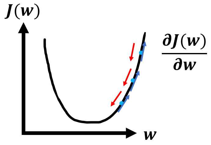
To start gradient descent, we can pick random values for $\mathbf{w}$ and calculate the loss $J(\mathbf{w})$ . We then take the derivative of the loss at $\mathbf{w}$ which tells us which direction our minimum is at. The blue arrows on the above graph are the derivative which point upwards since the derivative is positive. We want to head towards the minimum so we head opposite of the blue arrows (red arrows). Here's the general procedure for gradient descent:

Initialize $\mathbf{w}$ randomly
Repeat until minimum:

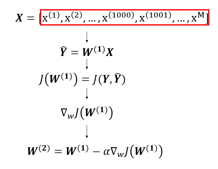
\mathbf{w}^{(k)} = \mathbf{w}^{(k-1)}-\alpha \nabla_{\mathbf{w}} J(\mathbf{w}^{(k-1)})

The learning rate, $\alpha$ , can be thought of as the step size for each iteration. The superscript, $k$ , represents the current iteration. I want to explain a bit more about the 2nd step "Repeat until minimum". This is the update step but when does it actually occur? That depends on whether we are using Stochastic Gradient Descent (SGD), Batch Gradient Descent, or Mini-Batch Gradient Descent. Firstly, let's define a term called epoch. An epoch is a pass through all $M$ samples in a dataset. In SGD, we update our weights, $\mathbf{w}$ , after each sample $m$ . Here's an example when using linear regression. Remember that the initial weights, $\mathbf{W}^{(1)}$ , are random.

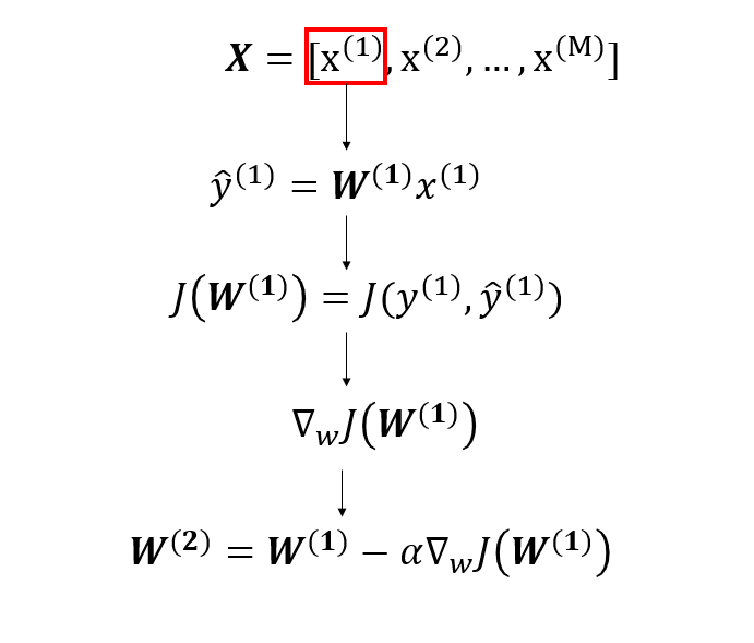
We take the first sample in our dataset and compute our predicted output, $\hat{y}$ , which is then fed into our loss function, $J$ . Afterwards, we calculate the derivative of the loss function and use it to update our value for the weights so we now have $\mathbf{W}^{(2)}$ . This is the weight we use when we repeat the above procedure for the next sample $x^{(2)}$ . We repeat the above procedure for each sample in our dataset. After we've done this for all of the samples, we've completed 1 epoch. We usually run multiple epochs until the values for our weights no longer change by a significant amount. In batch gradient descent, we go over the entire dataset before updating our weights.

Batch gradient descent ends up being less noisy than SGD but it takes a long time per each iteration. Mini-Batch gradient descent is a middle ground where we split our dataset into mini-batches that we use to perform updates.

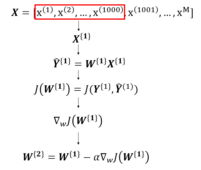
The mini-batches are represented by a curly brace. In the above example, the first 1000 examples are the first batch. We calculate our predictions using the first 1000 samples and sum our loss function for each sample in the batch. After we've gone through the entire batch, we then update our weights for the next batch.

Gradient descent is only one numerical way to find the minimum. There are many others such as RMSProp, Adam Optimization, and more. However, basic gradient descent will suffice for now.