The Navier-Stokes equations are fundamental equations describing fluid flow. I'll be going over the assumptions and math used to derive these equations. You should be
familiar with calculus, differential equations, and some basic physics as this makes up the bulk of the derivation.
Eulerian Description of Fluid Flow
The Navier-Stokes equations form the foundation of modern fluid mechanics. They are essentially conservation of momentum equations derived from Newton's
second law on a fluid. However, there are several concepts that need to be established on the journey towards Navier-Stokes. Let's first talk about the Eulerian
description of flow. Rather than following a particular fluid particle throughout its motion (Lagrange description), we will define an imaginary control volume and
evaluate the particles that pass in and out of this control volume. Therefore, instead of defining the velocity of a specific fluid particle, we define the
velocity field of the fluid that passes through the control volume.
V=u(x,y,z,t)i+v(x,y,z,t)j+w(x,y,z,t)k
Fluid elements passing through the control volume at a particular location and time will have the velocity defined above. The derivative of the velocity yields
acceleration, but this is only for Lagrangian particles. When using the Eulerian description, we must use the material derivative to calculate acceleration from
the velocity field. The material derivative is defined as:
DtDF=∂t∂F+(V⋅∇)F
The second term is the divergence of the velocity field which is defined as:
The material derivative offers a link between a Langragian and Eulerian descriptions of fluid flow.
Reynold's Transport Theorem (RTT)
In fluid mechanics, it is more common to work with control volumes rather than
a specific system of particles. In a system approach, we assume a closed system i.e. mass cannot cross our system boundary.
The control volume approach uses an open system where mass can go in and out of the boundaries. Most conservation laws are derived using a system rather than a control volume.
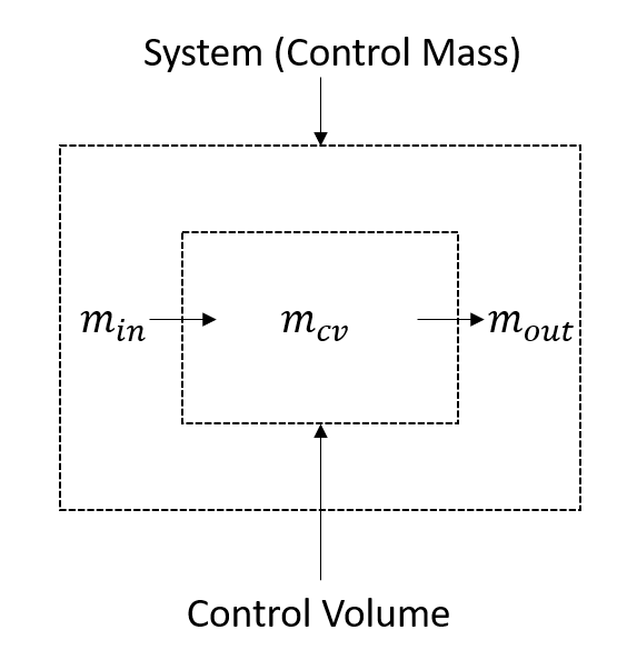
The above figure serves to illustrate the difference between a system and a control volume. The system encompasses all of the mass and will expand with it. The
control volume does not expand with the mass but it does record the mass entering and leaving its boundaries (along with the mass inside). Reynold's Transport
Theorem relates a system to a control volume. This allows us to derive conservation laws in terms of a control volume. We can see from the above figure that
the change in the system is equal to the change in the "stuff" inside the control volume plus the net change going in and out of the control volume.
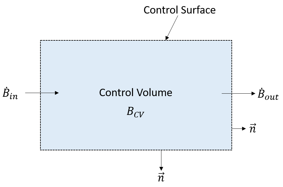
dtdBsys=dtdBCV+B˙out−B˙in
B simply represents an extensive property. An extensive property is a property that is proportional to the size or quantity of matter in a system such as mass,
volume, or entropy. An intensive property does not depend on the size or quantity of matter and is related to an extensive property via b=mB. The B˙
term can be re-written as bm˙ where m˙ is the mass flow rate. The mass flow rate can be further broken down into m˙=ρVA where ρ
is density, V is velocity, and A is area.
The net flux (B˙out−B˙in) can be written as:
B˙out−B˙in=∫CSbρV⋅ndA
n is the normal vector and its dot product with V ensures that we get the normal velocity. We integrate over the entire differential surface area
dA (inlet or outlet area). We write it this way so we can account for multiple inlets and outlets of differing sizes. For the control volume, BCV can be written as ∫cvbρdV where dV is the
differential volume. The original expression relating the system to the control volume is now:
dtdBsys=dtd∫CVbρdV+∫CSbρV⋅ndA
This is Reynold's Transport Theorem for a fixed control volume. For a moving control volume we simply replace the velocity in the above expression with the
relative velocity Vrel equal to:
Vrel=V−VCS
VCS is the velocity of the control surface.
Conservation of Mass
In Reynold's Transport Theorem, we looked at a generic extensive property called B and its intensive property b. In the case of mass conservation, the
extensive property is equal to mass (B=m) and therefore the intensive property is equal to b=mm=1. Let's write RTT in terms of mass:
dtdmsys=dtd∫CVρdV+∫CSρV⋅ndA
The left hand side of the above equation is the rate of change of mass in the system. However, we know that from a system perspective the mass does not change.
Unlike in a control volume, the system will continually transform along with the mass. Therefore, the change in mass of the system is equal to 0.
0=dtd∫CVρdV+∫CSρV⋅ndA
We can simplify the above expression by writing both terms as a volume integral.
0=∫CV[∂t∂ρ+∇⋅(ρV)]dVcv
In order for the above expression to equal 0, the expression in the integrand must also equal 0:
∂t∂ρ+∇⋅(ρV)=0
This is the general equation for conservation of mass, also known as the continuity equation. It can be further
expanded into the following using cartesian coordinates:
∂t∂ρ+∂x∂Vx+∂y∂Vy+∂z∂Vz=0
Conservation of Momentum
For this case, our extensive property is momentum (mV), so from RTT we have:
dtd(mV)sys=dtd∫CVVρdV+∫CSρVV⋅ndA
First, let's take a look at the left hand side. Our mass in the system is not changing so we can take out that term from the derivative. That leaves us with the
derivative of the velocity which is just acceleration. Therefore, we have mass times acceleration which is simply equal to the net force on the system.
∑F=dtd∫CVVρdV+∫CSρVV⋅ndA
The forces acting on the fluid includes surface (ex. pressure) and body (ex. gravity) forces. We can simplify the left hand side by assuming a Newtonian fluid with
the following stress tensor:
T=−(p+32μ∂xk∂Vk)δij+μ(∂xj∂Vi+∂xi∂Vj)
where p is pressure, μ is the dynamic viscosity of the fluid, and δij is the Kronecker delta. The Kronecker delta is equal to 1 when i=j and equal to 0
when i=j. If we assume that the fluid is incompressible (which is a reasonable assumption), then the stress tensor can be evaluated to the following.
The surface forces are inside a surface integral. b is the body forces per unit mass. The momentum expression is now:
∫CST⋅ndA+∫CVρbdV=dtd∫CVVρdV+∫CSρVV⋅ndA
We have terms in surface and volume integrals so we will write everything to be inside a volume integral using the divergence theorem.
∫CSρVV⋅ndA=∫CV∇⋅(ρVV)dV
∫CST⋅ndA=∫CV∇⋅TdV
Now we can rearrange everything inside a volume integral.
∫CV[∂t∂(ρV)+∇⋅(ρVV)−ρb−∇⋅T]dV=0
The expression inside the integrand must also equal zero for the above to hold true. Therefore, we can simplify to the following:
∂t∂(ρV)+∇⋅(ρVV)=ρb+∇⋅T
The expressions on the left can be expanded into the following.
∂t∂(ρV)=ρ∂t∂v+V∂t∂ρ
∇⋅(ρVV)=V∇⋅(ρV)+ρ(V⋅∇)V
Plugging the above back into our expression we have:
ρ∂t∂V+V∂t∂ρ+V∇⋅(ρV)+ρ(V⋅∇)V=ρb+∇⋅T
On the left hand side, we have the expression V∂t∂ρ+V∇⋅(ρV) which can be written as:
V(∂t∂ρ+∇⋅(ρV))
The expression in brackets is simply our conservation of mass expression from before which is equal to 0! So now we have:
ρ∂t∂V+ρ(V⋅∇)V=ρb+∇⋅T
The left hand side can be reduced even further. We can write ρ∂t∂V+ρ(V⋅∇)V as
ρ[∂t∂V+(V⋅∇)V] where the expression in brackets is the definition of the material
derivative. Therefore, we have:
ρDtDv=∇⋅T+ρb
If the only body force that acts on the CV is gravity then we can write b=g. Let's expand the above expression into cartesian coordinates.
The term in parentheses is simply 0 due to mass conservation and the squared partial derivatives are the Laplacian (∇2) of the u.
ρDtDu=∂x−∂P+μ∇2u+ρgx
The y and z terms can similarly be reduced to:
ρDtDv=∂y−∂P+μ∇2v+ρgy
ρDtDw=∂z−∂P+μ∇2w+ρgz
The three expressions can be written as one vector equation:
ρDtDV=−∇P+ρg+μ∇2V
This final expression is known as the Navier-Stokes equation. The above equation needs to be used in conjunction with the continuity equation when solving problems. This equation is a non-linear, 2nd-order partial differential equation. The solutions to this equation
are simplified cases with specific boundary conditions. There is no general solution to the above equation and it is in fact one of the millenium prize problems.